Sales Count Prediction per shops for the next month
Karim Mrezhoud
2019-10-31
- 0.1 Laod packages
- 1 Scores Versus Parameters: Resume of 6 runs
- 1.1 read & reduce files sizes
- 1.2 Merge dataframe & Explore
- 1.3 Item_id versus shop_id
- 1.4 How many shops and items?
- 1.5 How many items per shop_id?
- 1.6 What kind of items we have?
- 1.7 How many categories per shop?
- 1.8 Which categories that have more transactions?
- 1.9 Which Categories have few transactions
- 1.10 What is the goal?
- 1.11 How can identify ID in train dataset?
- 1.12 Other ID exist in train dataset and does not exist in test dataset?
- 1.13 ID with sales History
- 1.14 ID without sales past
- 1.15 Look for Item informations of ID without past sale
- 1.16 test ID versus sample_submission ID
- 1.17 Item_test versus item_train
- 1.18 Shops_test versus Shops_train
- 1.19 item_shop_test versus item_shop_train
- 1.20 History study of item_shop pairs that exist in test & train dataset
- 1.21 List of ID with History
- 1.22 Compute the monthly item_cnt_day
- 1.23 Plot the count of monthly sold ID with more that 100 transaction per month
- 1.24 What is ID 37296?
- 1.25 What is ID 46360
- 1.26 Trend of transactions per month
- 1.27 Trend of the amount of total item_prise purchased per shop
- 1.28 What about seasonality, trend, and cycle?
- 2 AutoCorrelation Function (ACF) and target lags
- 3 Feature Engineering
- 4 Notes: Parameters versus Features importance plots
- 5 Naive forecasting from this kernel
0.1 Laod packages
## ── Attaching packages ────────────────────────────────────────────────────────────────────── tidyverse 1.2.1 ──## ✔ ggplot2 3.2.1 ✔ purrr 0.3.2
## ✔ tibble 2.1.3 ✔ dplyr 0.8.3
## ✔ tidyr 1.0.0 ✔ stringr 1.4.0
## ✔ readr 1.3.1 ✔ forcats 0.4.0## ── Conflicts ───────────────────────────────────────────────────────────────────────── tidyverse_conflicts() ──
## ✖ dplyr::filter() masks stats::filter()
## ✖ dplyr::lag() masks stats::lag()##
## Attaching package: 'data.table'## The following objects are masked from 'package:dplyr':
##
## between, first, last## The following object is masked from 'package:purrr':
##
## transpose##
## Attaching package: 'lubridate'## The following objects are masked from 'package:data.table':
##
## hour, isoweek, mday, minute, month, quarter, second, wday,
## week, yday, year## The following object is masked from 'package:base':
##
## date##
## Attaching package: 'magrittr'## The following object is masked from 'package:purrr':
##
## set_names## The following object is masked from 'package:tidyr':
##
## extract##
## Attaching package: 'plotly'## The following object is masked from 'package:ggplot2':
##
## last_plot## The following object is masked from 'package:stats':
##
## filter## The following object is masked from 'package:graphics':
##
## layout##
## Attaching package: 'Matrix'## The following objects are masked from 'package:tidyr':
##
## expand, pack, unpack##
## Attaching package: 'xgboost'## The following object is masked from 'package:plotly':
##
## slice## The following object is masked from 'package:dplyr':
##
## slice1 Scores Versus Parameters: Resume of 6 runs
I tried several configuration to improve te score. The best one is the first one. I did not save to parameters For the best score, It was a testing For my first submission. After that I can not obtain less than 1.28 ‘:-))))’.
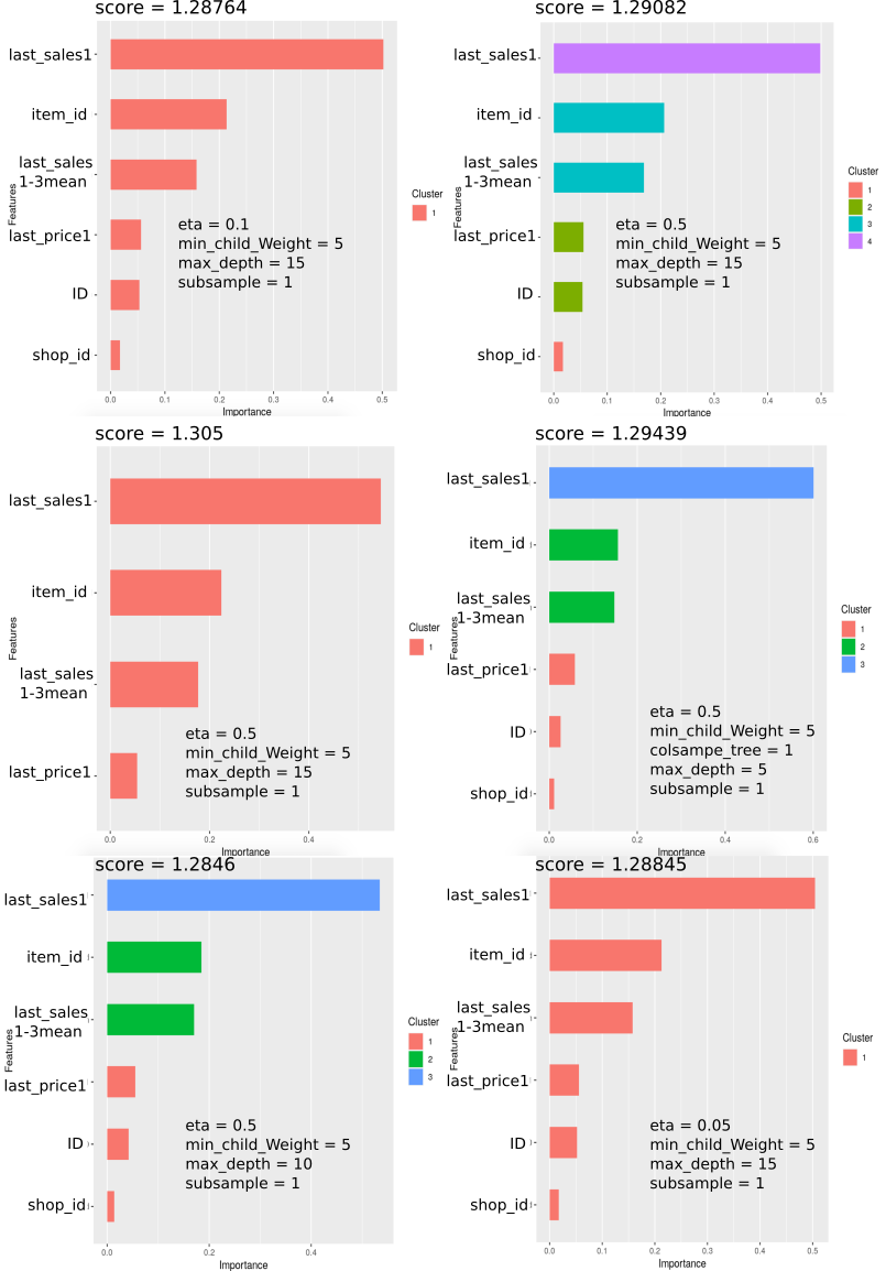
score Versus Params
1.1 read & reduce files sizes
# sales_train <- fread("sales_train.csv")
# test <- fread("test.csv")
# sample_submission <- fread("sample_submission.csv")
# item <- fread("items.csv")
# item_categories <- fread("item_categories.csv")
# shops <- fread("shops.csv")
#
# saveRDS(sales_train, "dataset/sales_train.rds")
# saveRDS(test, "dataset/test.rds")
# saveRDS(sample_submission, "dataset/sample_submission.rds")
# saveRDS(item, "dataset/item.rds")
# saveRDS(item_categories, "dataset/item_categories.rds")
# saveRDS(shops, "dataset/shops.rds")sales_train <- readRDS("dataset/sales_train.rds")
test <- readRDS("dataset/test.rds")
sample_submission <- readRDS("dataset/sample_submission.rds")
item <- readRDS("dataset/item.rds")
item_categories <- readRDS("dataset/item_categories.rds")
shops <- readRDS("dataset/shops.rds")1.1.1 Explore Sales train
## Observations: 2,935,849
## Variables: 6
## $ date <chr> "02.01.2013", "03.01.2013", "05.01.2013", "06.01.…
## $ date_block_num <int> 0, 0, 0, 0, 0, 0, 0, 0, 0, 0, 0, 0, 0, 0, 0, 0, 0…
## $ shop_id <int> 59, 25, 25, 25, 25, 25, 25, 25, 25, 25, 25, 25, 2…
## $ item_id <int> 22154, 2552, 2552, 2554, 2555, 2564, 2565, 2572, …
## $ item_price <dbl> 999.00, 899.00, 899.00, 1709.05, 1099.00, 349.00,…
## $ item_cnt_day <dbl> 1, 1, -1, 1, 1, 1, 1, 1, 1, 3, 2, 1, 1, 2, 1, 2, …1.1.2 Glimpse test
## Observations: 214,200
## Variables: 3
## $ ID <int> 0, 1, 2, 3, 4, 5, 6, 7, 8, 9, 10, 11, 12, 13, 14, 15, 16…
## $ shop_id <int> 5, 5, 5, 5, 5, 5, 5, 5, 5, 5, 5, 5, 5, 5, 5, 5, 5, 5, 5,…
## $ item_id <int> 5037, 5320, 5233, 5232, 5268, 5039, 5041, 5046, 5319, 50…1.1.3 Glimpse item
## Observations: 22,170
## Variables: 3
## $ item_name <chr> "! ВО ВЛАСТИ НАВАЖДЕНИЯ (ПЛАСТ.) D", "!…
## $ item_id <int> 0, 1, 2, 3, 4, 5, 6, 7, 8, 9, 10, 11, 12, 13, 1…
## $ item_category_id <int> 40, 76, 40, 40, 40, 40, 40, 40, 40, 40, 40, 40,…1.1.4 Glimpse item_categories
## Observations: 84
## Variables: 2
## $ item_category_name <chr> "PC - Гарнитуры/Наушники", "Аксессуары - PS2"…
## $ item_category_id <int> 0, 1, 2, 3, 4, 5, 6, 7, 8, 9, 10, 11, 12, 13,…1.1.5 Glimpse shops
## Observations: 60
## Variables: 2
## $ shop_name <chr> "!Якутск Орджоникидзе, 56 фран", "!Якутск ТЦ \"\"Центр…
## $ shop_id <int> 0, 1, 2, 3, 4, 5, 6, 7, 8, 9, 10, 11, 12, 13, 14, 15, …1.1.6 Glimpse submission file
## Observations: 214,200
## Variables: 2
## $ ID <int> 0, 1, 2, 3, 4, 5, 6, 7, 8, 9, 10, 11, 12, 13, 14,…
## $ item_cnt_month <dbl> 0.5, 0.5, 0.5, 0.5, 0.5, 0.5, 0.5, 0.5, 0.5, 0.5,…1.2 Merge dataframe & Explore
train <- sales_train %>%
left_join(item, by = "item_id") %>%
left_join(item_categories, by = "item_category_id") %>%
left_join(shops, by = "shop_id")
rm(sales_train, item, item_categories, shops)
invisible(gc())
DataExplorer::plot_intro(train)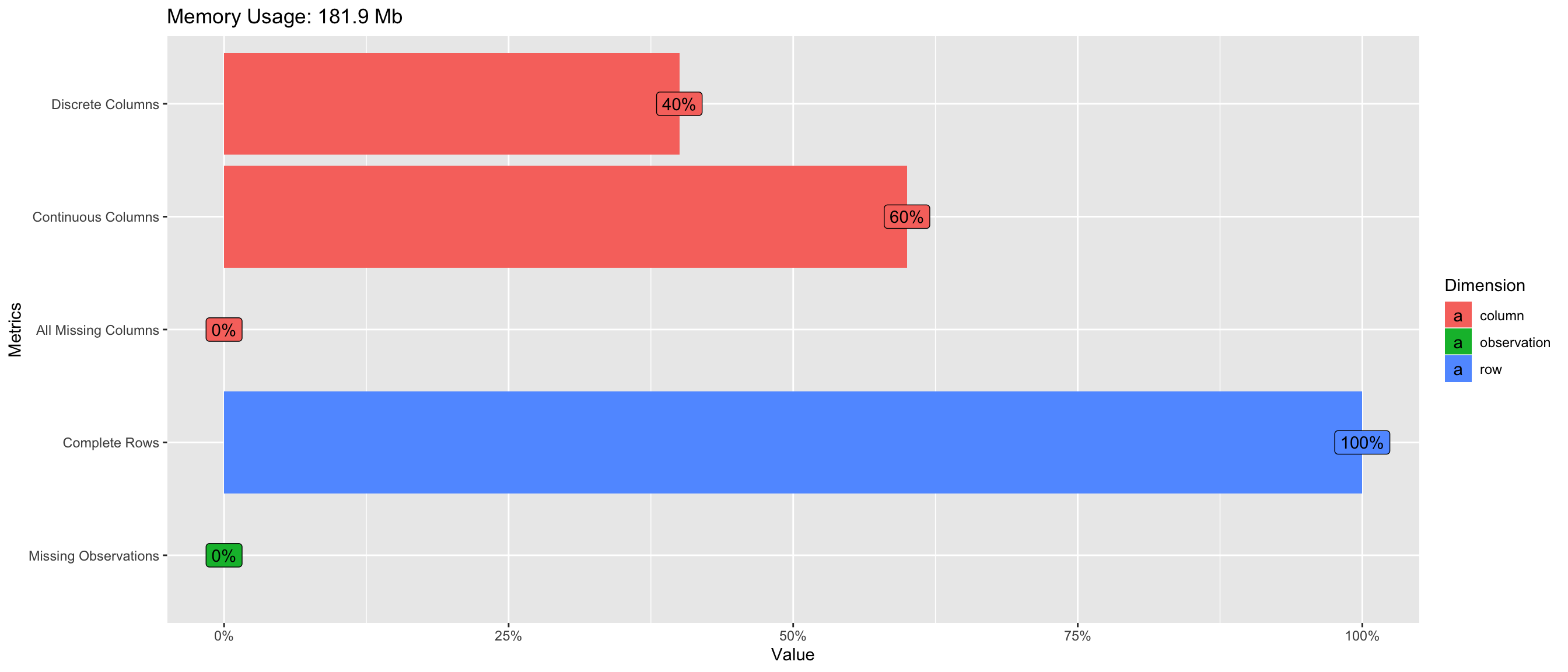
1.2.1 Explore correlation
## Warning in dummify(data, maxcat = maxcat): Ignored all discrete features
## since `maxcat` set to 20 categories!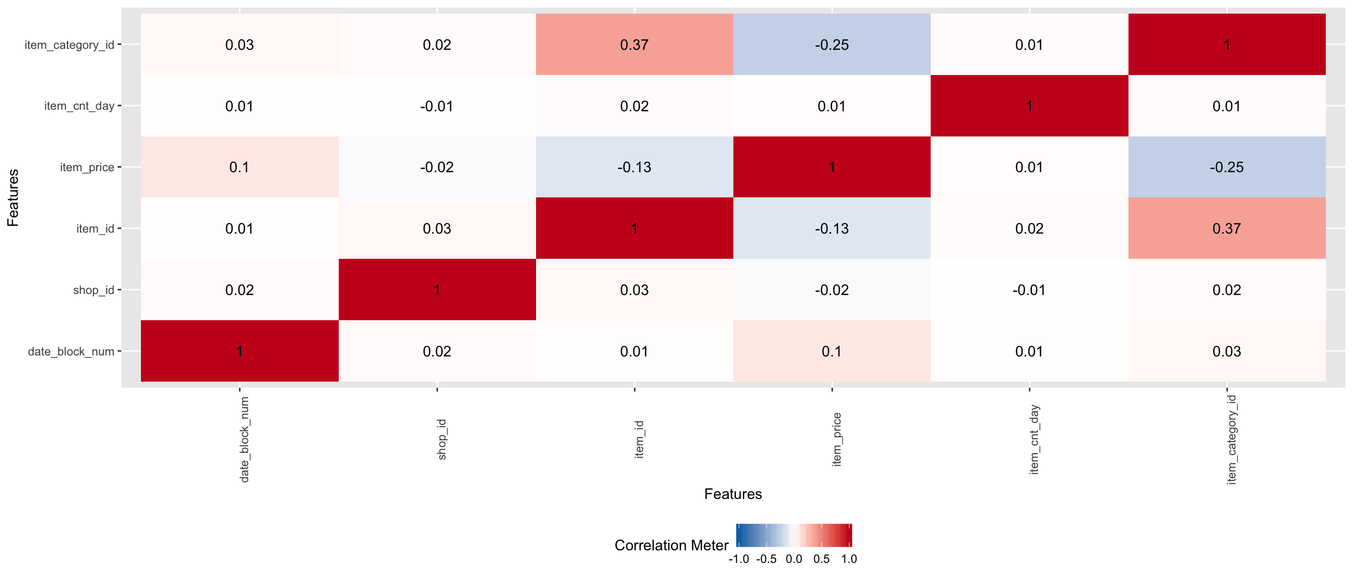
1.3 Item_id versus shop_id
## shop_id item_id
## 1 59 22154
## 2 25 2552
## 3 25 2552
## 4 25 2554
## 5 25 2555
## 6 25 2564- one
shop_idcan has multipleitem_id - the same formula
f(shop_id,item_id)is repeated several time during the period.
1.4 How many shops and items?
## [1] "In test data, tere is : 42 shops"## [1] "In test data there is: 5100 items"1.5 How many items per shop_id?
p <- train %>%
mutate(date = dmy(date)) %>%
mutate(shop_id = as.character(as.factor(shop_id))) %>%
select(date, shop_id, item_id) %>%
group_by(date,shop_id) %>%
summarise(n_items = sum(n_distinct(item_id))) %>%
ggplot()+
aes(x = date, y = n_items, fill = shop_id) +
geom_col() +
scale_x_date(date_labels="%b %y",date_breaks ="1 month") +
theme( axis.text.x = element_text(angle=45, hjust=1, vjust=0.9))
ggplotly(p)- There is some season of the freq items sales per shop
- this saeson is related to date.
- always shops with orange color have sold more items than shops with pink color. This means that for example shops 0, 1, 2 have more items that shops 54, 55, 56 during any date during this dataset.
1.6 What kind of items we have?
train %>%
select(item_category_id, item_name) %>%
group_by(item_category_id) %>%
count() %>%
arrange(item_category_id) %>% summary()## item_category_id n
## Min. : 0.00 Min. : 1
## 1st Qu.:20.75 1st Qu.: 1475
## Median :41.50 Median : 6918
## Mean :41.50 Mean : 34951
## 3rd Qu.:62.25 3rd Qu.: 26608
## Max. :83.00 Max. :564652- It seems like Fnac shop in Russia
- there is 84 caterogies and 21807 items descriptions
- The freq can increase until 31340 but the mean is about 134 items and the median is about 32 items.
1.7 How many categories per shop?
Get idea about the size of shops.
train %>%
select(shop_id, item_category_id) %>%
group_by(shop_id) %>%
summarise(n_cat = n_distinct(item_category_id)) %>%
ggplot() +
aes(x = shop_id, y =n_cat, fill= n_cat ) %>%
geom_col()+
theme( axis.text.x = element_text(angle=45, hjust=1, vjust=0.9))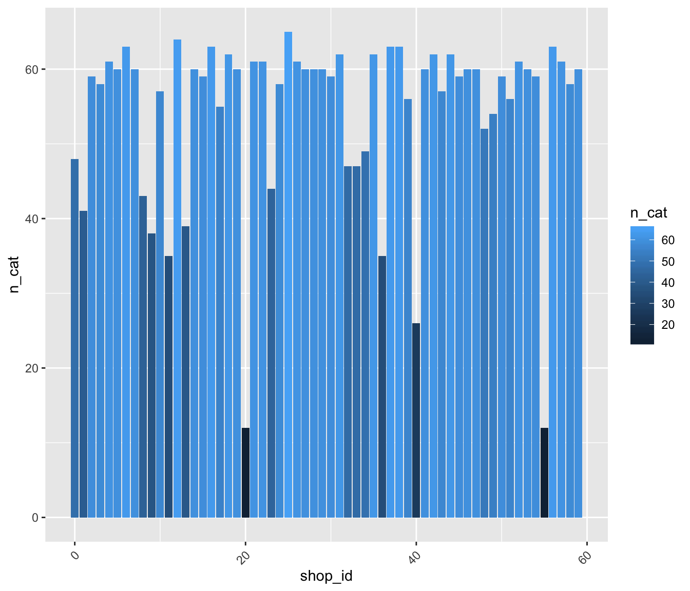 * Most shops have more than 40 categories.
1.8 Which categories that have more transactions?
train %>%
group_by(item_category_id) %>%
summarise(n_transactions = sum(item_cnt_day)) %>%
ggplot() +
aes(x= as.factor(item_category_id), y = n_transactions) +
geom_col() +
theme( axis.text.x = element_text(angle=45, hjust=1, vjust=0.9))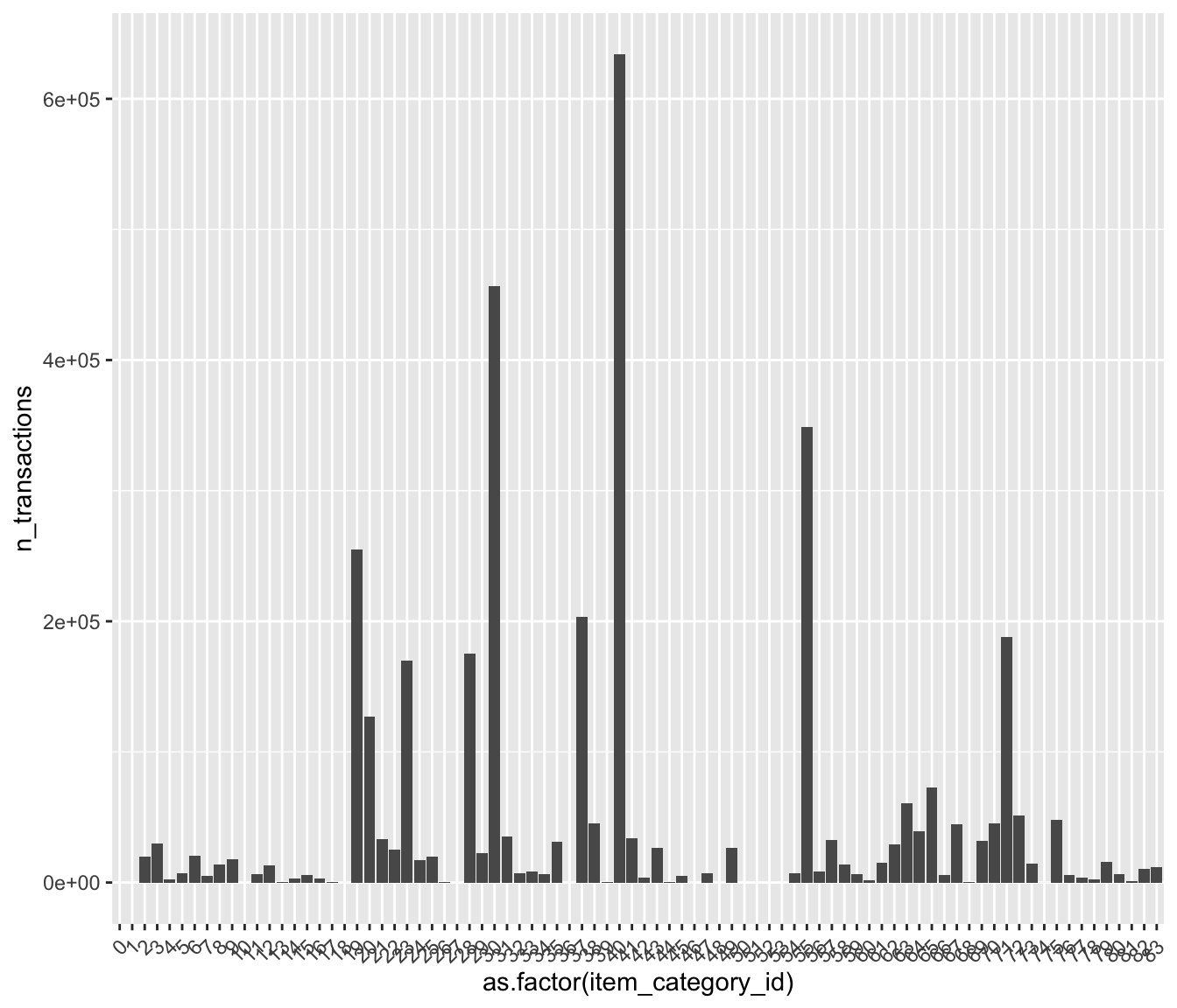 * caterogies: 40 has the first rank. After: 30, 55, 19, 37, 71, 28, 23. * some categories have zero or few solds.
1.9 Which Categories have few transactions
train %>%
group_by(item_category_id) %>%
summarise(n_transactions = sum(item_cnt_day)) %>%
arrange(n_transactions) %>%
filter(n_transactions < 1000)## # A tibble: 20 x 2
## item_category_id n_transactions
## <int> <dbl>
## 1 10 1
## 2 51 1
## 3 1 2
## 4 0 3
## 5 50 3
## 6 52 3
## 7 53 3
## 8 48 6
## 9 27 8
## 10 18 11
## 11 46 15
## 12 36 22
## 13 74 59
## 14 26 114
## 15 68 129
## 16 44 252
## 17 17 295
## 18 13 357
## 19 39 646
## 20 81 965- Maybe we can consider that categories with less that 1000 sold during the study are not important for prediction.
We can play with question and answers and plot a lot of graphes…. But
1.10 What is the goal?
Submission file has ID and item_cnt_day columns. The ID is a (Shop, Item) tuple that we can find in test file.
1.11 How can identify ID in train dataset?
Each ID is an unique cancatenation of shop_id and item_id.
## ID shop_id item_id IDx
## 1 0 5 5037 5_5037
## 2 1 5 5320 5_5320
## 3 2 5 5233 5_5233
## 4 3 5 5232 5_5232
## 5 4 5 5268 5_5268
## 6 5 5 5039 5_50391.12 Other ID exist in train dataset and does not exist in test dataset?
IDx minus ID is IDs that do not exist in submission file
p <- train %>%
mutate(IDx = paste(shop_id, item_id, sep = "_")) %>%
full_join(test, by= c("shop_id","item_id" ,"IDx")) %>%
select(date_block_num ,shop_id, item_id, IDx, ID, item_cnt_day) %>%
mutate(item_id = as.factor(as.character(item_id))) %>%
filter(is.na(ID)) %>%
group_by(date_block_num, shop_id) %>%
#summarise(item_cnt_month = sum(item_cnt_day)) %>%
summarise(n_item = n_distinct(item_id)) %>%
ggplot() +
aes(x = date_block_num, y = n_item, fill = shop_id) +
geom_col()
ggplotly(p)- The items without ID decrease during the time series
1.13 ID with sales History
p1 <- train %>%
mutate(IDx = paste(shop_id, item_id, sep = "_")) %>%
full_join(test, by= c("shop_id","item_id" ,"IDx")) %>%
select(date_block_num ,shop_id, item_id, IDx, ID, item_cnt_day) %>%
mutate(item_id = as.factor(as.character(item_id))) %>%
filter(!is.na(ID)) %>%
filter(!is.na(date_block_num)) %>%
group_by(date_block_num, shop_id) %>%
summarise(n_item = n_distinct(item_id)) %>%
ggplot() +
aes(x = date_block_num, y = n_item, fill = shop_id) +
geom_col()
ggplotly(p1)1.14 ID without sales past
train %>%
mutate(IDx = paste(shop_id, item_id, sep = "_")) %>%
full_join(test, by= c("shop_id","item_id" ,"IDx")) %>%
select(date_block_num ,item_category_id, shop_id, item_id, IDx, ID, item_cnt_day) %>%
#mutate(item_id = as.factor(as.character(item_id))) %>%
#mutate(shop_id = as.factor(as.character(shop_id))) %>%
filter(!is.na(ID)) %>%
filter(is.na(date_block_num)) %>%
select(ID) %>%
n_distinct()## [1] 102796OOO! There is 102796/214200 (48%) of ID in test and in train but do not have past sales.
1.15 Look for Item informations of ID without past sale
train %>%
mutate(IDx = paste(shop_id, item_id, sep = "_")) %>%
full_join(test, by= c("shop_id","item_id" ,"IDx")) %>%
filter(!is.na(ID)) %>%
filter(is.na(date_block_num)) %>%
summary## date date_block_num shop_id item_id
## Length:102796 Min. : NA Min. : 2.00 Min. : 30
## Class :character 1st Qu.: NA 1st Qu.:15.00 1st Qu.: 5653
## Mode :character Median : NA Median :36.00 Median :11572
## Mean :NaN Mean :31.91 Mean :11166
## 3rd Qu.: NA 3rd Qu.:48.00 3rd Qu.:16140
## Max. : NA Max. :59.00 Max. :22167
## NA's :102796
## item_price item_cnt_day item_name item_category_id
## Min. : NA Min. : NA Length:102796 Min. : NA
## 1st Qu.: NA 1st Qu.: NA Class :character 1st Qu.: NA
## Median : NA Median : NA Mode :character Median : NA
## Mean :NaN Mean :NaN Mean :NaN
## 3rd Qu.: NA 3rd Qu.: NA 3rd Qu.: NA
## Max. : NA Max. : NA Max. : NA
## NA's :102796 NA's :102796 NA's :102796
## item_category_name shop_name IDx ID
## Length:102796 Length:102796 Length:102796 Min. : 1
## Class :character Class :character Class :character 1st Qu.: 57300
## Mode :character Mode :character Mode :character Median :117206
## Mean :112474
## 3rd Qu.:166205
## Max. :214198
## - Not informations about ID without Sales past.
1.16 test ID versus sample_submission ID
## ID shop_id item_id IDx
## Min. : 0 Min. : 2.00 Min. : 30 Length:214200
## 1st Qu.: 53550 1st Qu.:16.00 1st Qu.: 5382 Class :character
## Median :107100 Median :34.50 Median :11203 Mode :character
## Mean :107100 Mean :31.64 Mean :11019
## 3rd Qu.:160649 3rd Qu.:47.00 3rd Qu.:16072
## Max. :214199 Max. :59.00 Max. :22167
## item_cnt_month
## Min. :0.5
## 1st Qu.:0.5
## Median :0.5
## Mean :0.5
## 3rd Qu.:0.5
## Max. :0.5- Identical ID are present in test and Sample_submission.
The goal is to predict a monthly amount of item_cnt_dat
1.17 Item_test versus item_train
item_test <- unique(test$item_id)
item_train <- unique(train$item_id)
item_in_test_in_train <- item_test[item_test %in% item_train]
item_in_test_not_train <- item_test[!item_test %in% item_train]
paste("there is sales history of ", round((length(item_in_test_in_train)*100)/length(item_test)), "% of items in dataset test" )## [1] "there is sales history of 93 % of items in dataset test"1.18 Shops_test versus Shops_train
shop_test <- unique(test$shop_id)
shop_train <- unique(train$shop_id)
shop_in_test_in_train <- shop_test[shop_test %in% shop_train]
shop_test_not_train <- shop_test[!shop_test %in% shop_train]
paste("there is sales history of ",round((length(shop_in_test_in_train)*100)/length(shop_test)), "% of shops in test dataset " )## [1] "there is sales history of 100 % of shops in test dataset "1.19 item_shop_test versus item_shop_train
item_shop_test <- test %>% mutate(IDx = paste(shop_id, item_id, sep = "_")) %>% select(IDx) %>% as.list
item_shop_train <- train %>% mutate(IDx = paste(shop_id, item_id, sep = "_")) %>% select(IDx) %>% as.list
item_shop_in_test_in_train <- item_shop_test$IDx[item_shop_test$IDx %in% item_shop_train$IDx]
item_shop_in_test_not_train <- item_shop_test$IDx[!item_shop_test$IDx %in% item_shop_train$IDx]
paste("there is sales history of", round((length(item_shop_in_test_in_train)*100)/length(item_shop_test$IDx)), "% of item_shop pairs in test dataset")## [1] "there is sales history of 52 % of item_shop pairs in test dataset"1.20 History study of item_shop pairs that exist in test & train dataset
train_ID_with_history <- train %>%
mutate(IDx = paste(shop_id, item_id, sep = "_")) %>%
full_join(test, by= c("shop_id","item_id" ,"IDx")) %>%
filter( IDx %in% item_shop_in_test_in_train ) %>%
select(date, date_block_num, ID, item_cnt_day, item_price) %>%
group_by(date_block_num, ID) %>%
summarise(item_cnt_month = sum(item_cnt_day))
train_ID_with_history %>% head(20)## # A tibble: 20 x 3
## # Groups: date_block_num [1]
## date_block_num ID item_cnt_month
## <int> <int> <dbl>
## 1 0 5122 1
## 2 0 5127 3
## 3 0 5142 2
## 4 0 5143 9
## 5 0 5152 1
## 6 0 5169 4
## 7 0 5185 2
## 8 0 5186 2
## 9 0 5254 1
## 10 0 5308 3
## 11 0 5331 3
## 12 0 5358 1
## 13 0 5374 20
## 14 0 5407 1
## 15 0 5445 4
## 16 0 5496 4
## 17 0 5505 1
## 18 0 5515 12
## 19 0 5520 1
## 20 0 5523 11.21 List of ID with History
ID_in_test_in_train <- train %>%
mutate(IDx = paste(shop_id, item_id, sep = "_")) %>%
full_join(test, by= c("shop_id","item_id" ,"IDx")) %>%
filter( IDx %in% item_shop_in_test_in_train ) %>%
select(ID) %>% unique
ID_in_test_in_train$ID %>% head(100)## [1] 150983 56520 56539 56666 57021 60179 59134 59196 56632 56634
## [11] 56496 59067 59053 56505 60844 60006 59147 56766 57236 56653
## [21] 56654 56669 58228 57515 61179 60043 56523 59197 56530 56652
## [31] 58230 60237 57435 59176 58138 58140 60136 56706 60841 58825
## [41] 58131 60840 57445 57833 56595 59188 59104 58135 56673 58134
## [51] 60842 58136 58216 58226 56639 58821 56515 59070 58128 57391
## [61] 59139 56708 60020 59634 59636 59638 59639 59641 59642 59625
## [71] 59620 59624 58559 58579 58945 57068 57069 58554 60134 57136
## [81] 60015 58561 58951 60045 56127 57960 57961 57225 57118 61099
## [91] 58720 58632 59585 57073 57989 56141 56152 59615 56142 561431.22 Compute the monthly item_cnt_day
train %>%
mutate(IDx = paste(shop_id, item_id, sep = "_")) %>%
left_join(test, by= c("shop_id","item_id" ,"IDx")) %>%
select(date, date_block_num ,shop_id, item_id, IDx, ID, item_cnt_day) %>%
na.omit(ID) %>%
mutate(date_block_num = as.factor(date_block_num),ID= as.factor(ID)) %>%
group_by(date_block_num, ID) %>%
summarise(item_cnt_month = sum(item_cnt_day)) %>%
arrange(desc(item_cnt_month)) %>%
head()## # A tibble: 6 x 3
## # Groups: date_block_num [4]
## date_block_num ID item_cnt_month
## <fct> <fct> <dbl>
## 1 33 37296 2253
## 2 11 46360 1305
## 3 23 46360 1209
## 4 11 56560 1066
## 5 24 36160 1000
## 6 23 56560 997- During month 33 (Nov 2015) we have 2253 transactions of ID 37296. Reminber ID is shop_item encoding.
1.23 Plot the count of monthly sold ID with more that 100 transaction per month
p <- train %>%
mutate(IDx = paste(shop_id, item_id, sep = "_")) %>%
left_join(test, by= c("shop_id","item_id" ,"IDx")) %>%
select(date, date_block_num ,shop_id, item_id, IDx, ID, item_cnt_day) %>%
na.omit(ID) %>%
mutate(date_block_num = as.factor(date_block_num), ID= as.factor(ID)) %>%
group_by(date_block_num, ID) %>%
summarise(item_cnt_month = sum(item_cnt_day)) %>%
filter(item_cnt_month > 100) %>%
ggplot() +
aes(x = date_block_num, y =item_cnt_month, fill = ID) +
geom_col()
# theme( axis.text.x = element_text(angle=45, hjust=1, vjust=0.9))
ggplotly(p)The goal is to predict the next bar plot of December 2015. There is 214200 ID in test and sample_submission.
1.24 What is ID 37296?
- Доставка до пункта выдачи (Boxberry): Delivery to pick-up point (Boxberry)
- Доставка товара: Delivery of goods
- Интернет-магазин ЧС: Emergency Shop Online
train %>%
mutate(IDx = paste(shop_id, item_id, sep = "_")) %>%
left_join(test, by= c("shop_id","item_id" ,"IDx")) %>%
na.omit(ID) %>%
filter(ID == "37296") %>%
ggplot() +
aes(x=date_block_num, y= item_price, color = item_price) +
geom_point()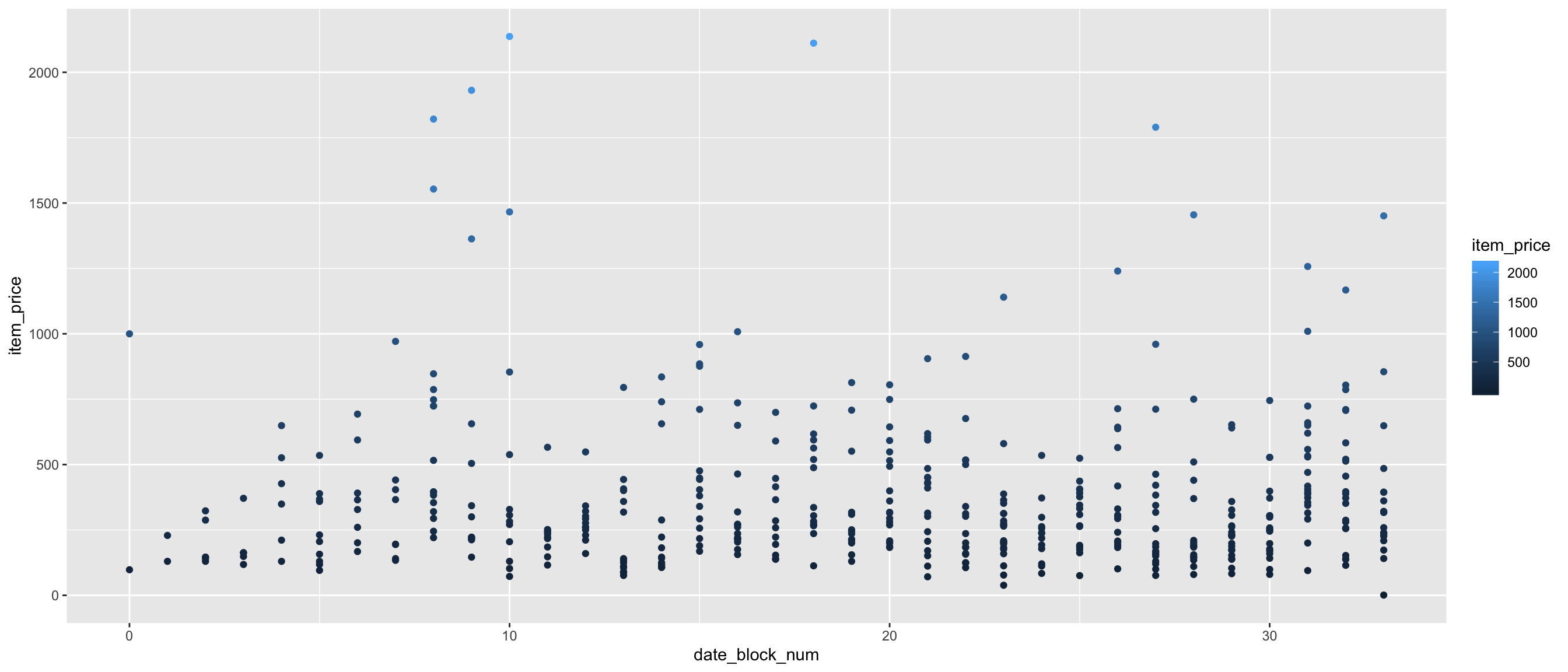 The goal on this plot is to check if the price of the Boxberry is in sold or not during the last months.
1.25 What is ID 46360
- Фирменный пакет майка 1С Интерес белый (34x42) 45 мкм: Chemise de paquet entreprise 1C intérêt blanc (34 * 42) 45 microns
- Подарки - Сумки, Альбомы, Коврики д/мыши: Cadeaux - Sacs, Albums, Tapis de souris
- Подарки - Сумки, Альбомы, Коврики д/мыши: Cadeaux - Sacs, Albums, Tapis de souris
- Москва ТЦ "“Семеновский”“: Centre commercial de Moscou”" Semenovsky ""
p <- train %>%
mutate(IDx = paste(shop_id, item_id, sep = "_")) %>%
left_join(test, by= c("shop_id","item_id" ,"IDx")) %>%
na.omit(ID) %>%
filter(ID == "46360") %>%
ggplot() +
aes(x=date_block_num, y= item_price, color = item_price) +
geom_point()
p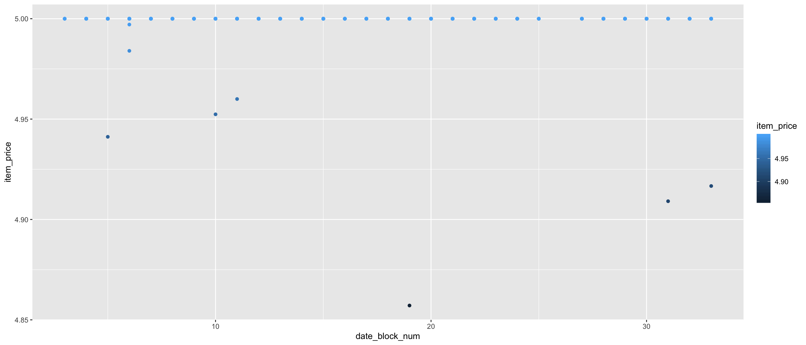 The decrease of item_cnt_day is not related to price.
1.26 Trend of transactions per month
p <- train %>%
mutate(IDx = paste(shop_id, item_id, sep = "_")) %>%
left_join(test, by= c("shop_id","item_id" ,"IDx")) %>%
select(date, date_block_num ,shop_id, ID, item_cnt_day) %>%
mutate(date_block_num = as.factor(date_block_num), shop_id= as.factor(shop_id)) %>%
na.omit(ID) %>%
group_by(date_block_num, shop_id) %>%
summarise(transactions = sum(item_cnt_day)) %>%
ggplot() +
aes(x = date_block_num, y = transactions, fill = shop_id) +
geom_col()
ggplotly(p)- The trend of total transaction is in increase.
1.27 Trend of the amount of total item_prise purchased per shop
p <- train %>%
mutate(IDx = paste(shop_id, item_id, sep = "_")) %>%
full_join(test, by= c("shop_id","item_id" ,"IDx")) %>%
select(date, date_block_num ,shop_id, ID, item_price,item_cnt_day) %>%
mutate(date_block_num = as.factor(date_block_num), shop_id= as.factor(shop_id)) %>%
#na.omit(ID) %>%
mutate(Amount = ifelse((item_cnt_day <= 0)|(item_price <= 0), 0, item_price*item_cnt_day)) %>%
group_by(date_block_num, shop_id) %>%
summarise(total_amount = sum(Amount)) %>%
ggplot() +
aes(x = date_block_num, y =total_amount, fill = shop_id) +
geom_col()## Warning: Factor `date_block_num` contains implicit NA, consider using
## `forcats::fct_explicit_na`## Warning: Removed 42 rows containing missing values (position_stack).Also, I think there is an increase trend of the total amount per month.
1.28 What about seasonality, trend, and cycle?
rucm package can extract seasonal characteristics from time series. ### Monthly Transactions Number trend
## Loading required package: zoo##
## Attaching package: 'zoo'## The following objects are masked from 'package:base':
##
## as.Date, as.Date.numeric##
## Attaching package: 'xts'## The following objects are masked from 'package:data.table':
##
## first, last## The following objects are masked from 'package:dplyr':
##
## first, last## Loading required package: KFASdf <- train %>%
mutate(IDx = paste(shop_id, item_id, sep = "_")) %>%
full_join(test, by= c("shop_id","item_id" ,"IDx")) %>%
filter( IDx %in% item_shop_in_test_in_train ) %>%
select(date, date_block_num, ID, item_cnt_day, item_price) %>%
group_by(date_block_num, ID) %>%
summarise(item_cnt_month = sum(item_cnt_day))
## convert df as time series (ts)
Transactions <- ts(df$item_cnt_month/10,
start = 0,
end = 33,
frequency = 1)
model_trans <- ucm(formula = Transactions~0, data = Transactions, level = TRUE,season = TRUE, season.length = 3, slope = TRUE)
{plot(Transactions) +
## plot
lines(model_trans$s.level, col = "blue") +
### plot Prediction Transactions number for the x N months
lines(predict(model_trans$model, n.ahead = 10), col = "red")+
abline(reg=lm(Transactions~time(Transactions)), col = "green")}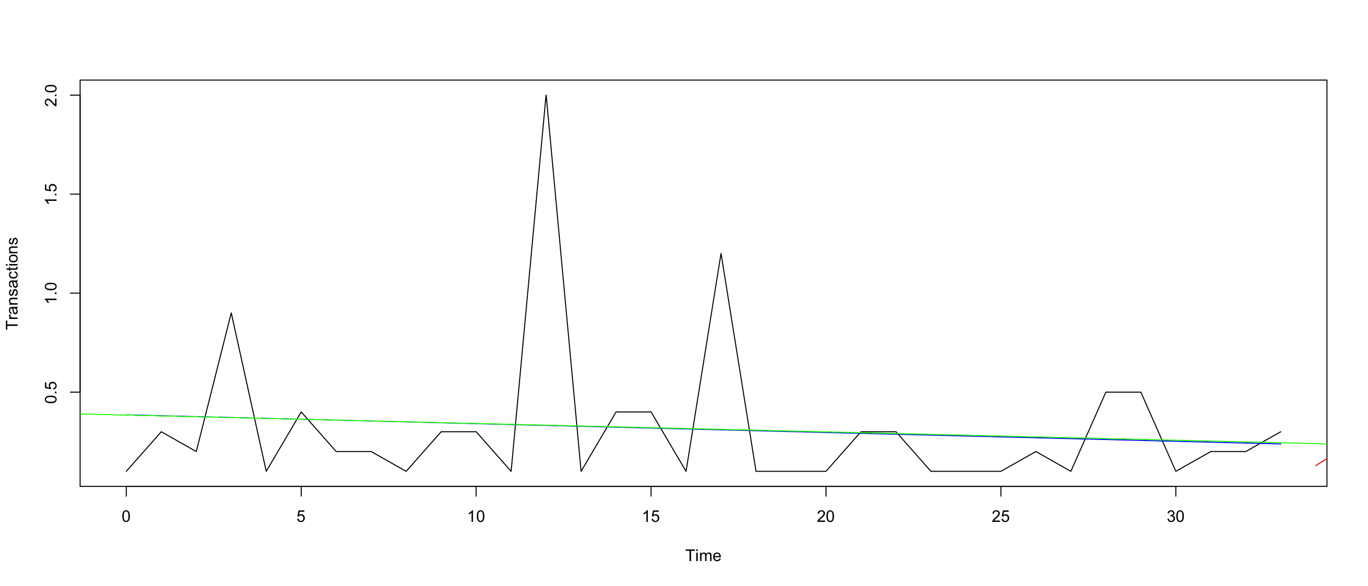
## integer(0)1.28.1 ggplot prediction of the number of transaction for the next Months
pred <- predict(model_trans$model, n.ahead = 17)
pred_df <- cbind(time =34:50, as.data.frame(pred))
ggplot(df) +
geom_line(aes(x = date_block_num , y = item_cnt_month)) +
geom_line(data = pred_df, aes(x = time, y = fit), color = "red") +
geom_abline(slope = model_trans$s.slope, intercept = 2000, color = "blue")## Don't know how to automatically pick scale for object of type ts. Defaulting to continuous.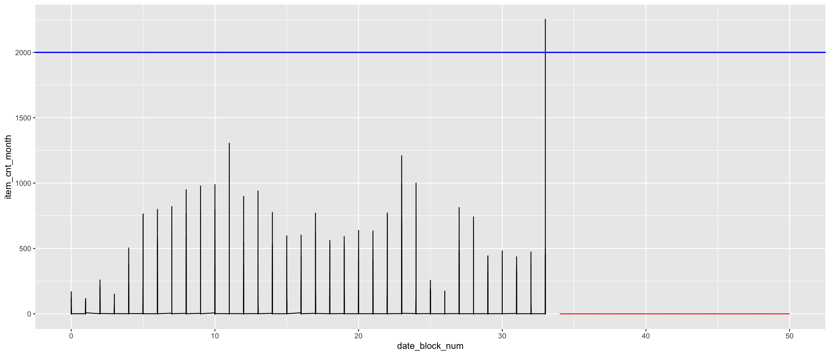 * This plot does not take in account the seasonality.
1.28.2 Monthly Amount Trend
df <- train %>%
mutate(IDx = paste(shop_id, item_id, sep = "_")) %>%
full_join(test, by= c("shop_id","item_id" ,"IDx")) %>%
filter( IDx %in% item_shop_in_test_in_train ) %>%
select(date, date_block_num ,shop_id, ID, item_price,item_cnt_day) %>%
group_by(date_block_num) %>%
summarise(Mean_Monthly_Amount = sum(item_price)/sum(item_cnt_day))
## convert df as time series (ts)
Mean_Monthly_Amount <- ts(df$Mean_Monthly_Amount,
start = 0,
end = 33,
frequency = 1)
model_amount <- ucm(formula = Mean_Monthly_Amount~0,
data = Mean_Monthly_Amount,
level = TRUE, season = TRUE,
season.length = 3, slope = TRUE)
{plot(Mean_Monthly_Amount)
lines(model_amount$s.level, col = "blue")+
abline(reg=lm(Mean_Monthly_Amount~time(Mean_Monthly_Amount)), col = "green")}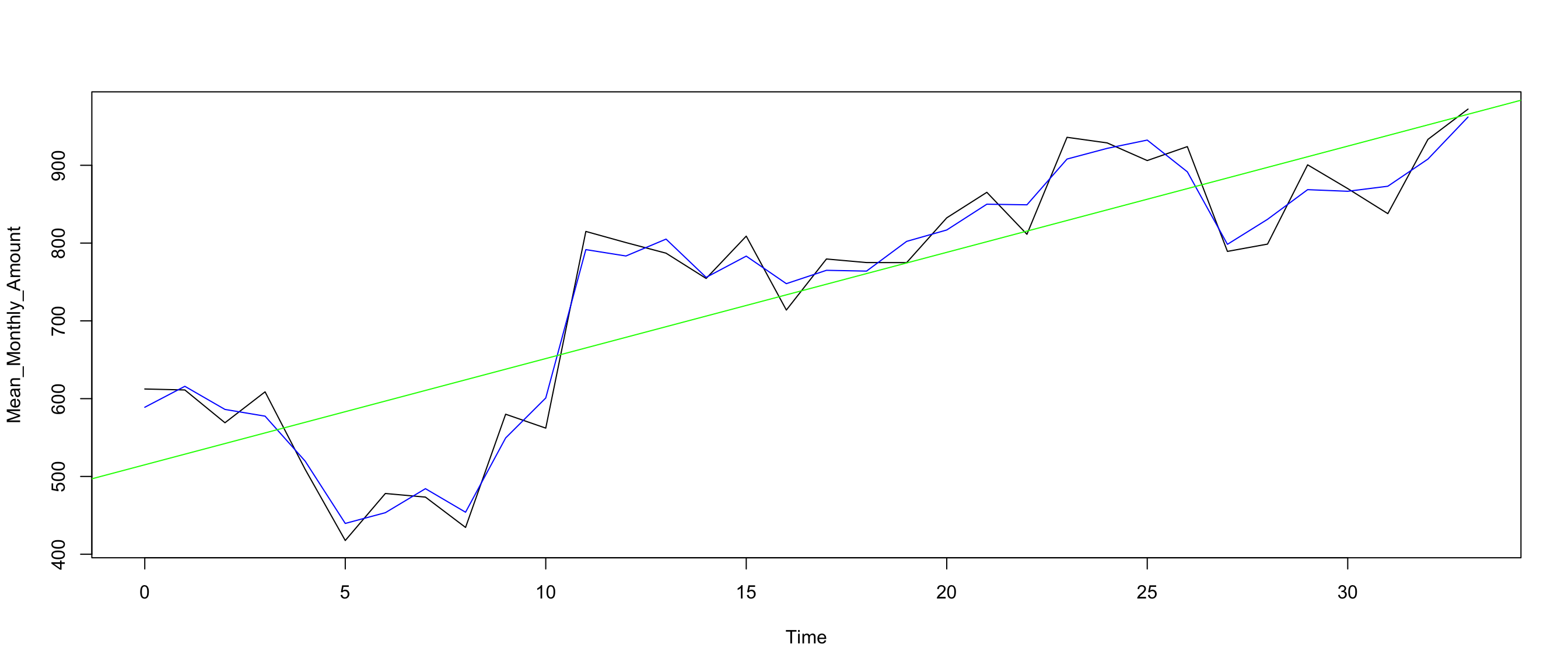
## integer(0)pred_amount <- predict(model_amount$model, n.ahead = 17)
pred_amount_df <- cbind(time =34:50, as.data.frame(pred_amount))
ggplot(df) +
geom_line(aes(x = date_block_num, y = Mean_Monthly_Amount)) +
geom_line(data = pred_amount_df, aes(x = time, y = fit), color = "red") +
geom_abline(slope = model_amount$s.slope, intercept = 400,color = "blue")## Don't know how to automatically pick scale for object of type ts. Defaulting to continuous.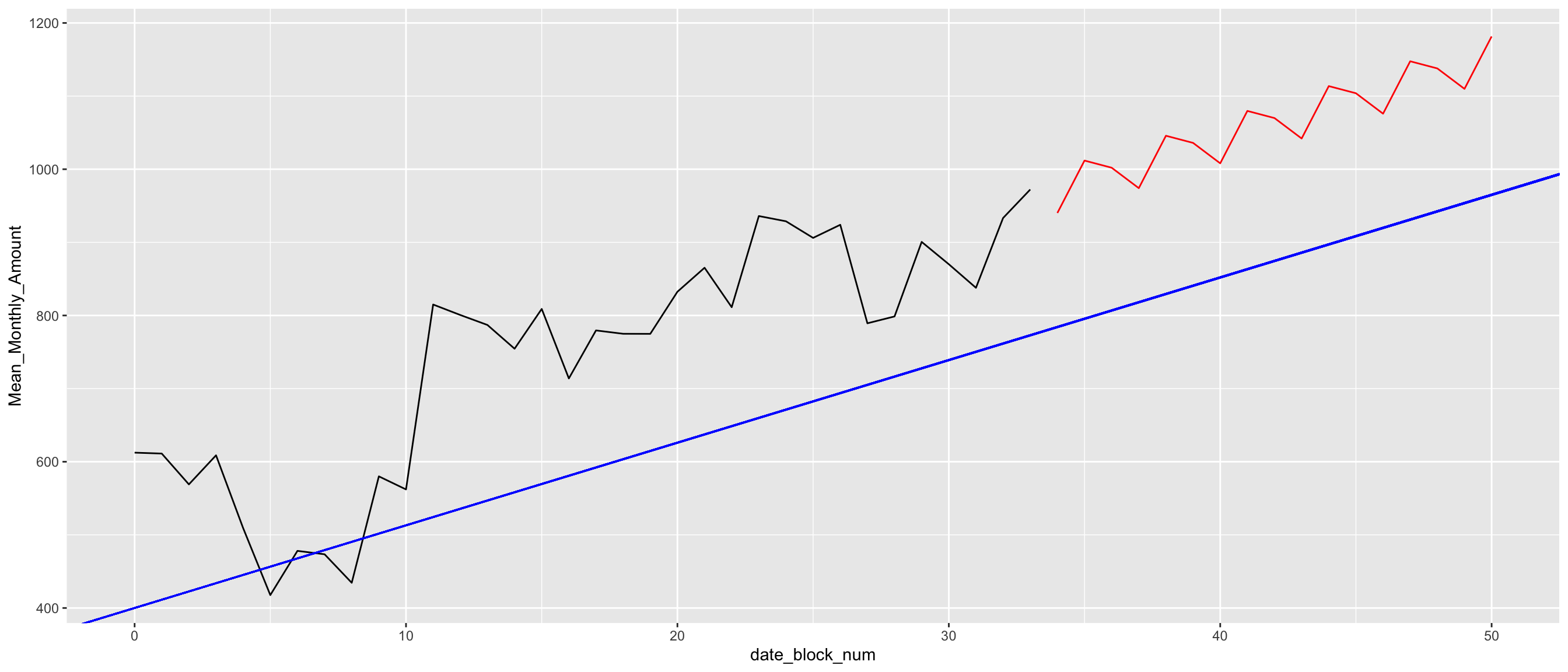
2 AutoCorrelation Function (ACF) and target lags
2.1 Function to get best lags of each ID
#library(xts)
## df must have ID, date_block_num, item_cnt_month columns
get_lag <- function(id, df, lag.max = 12, plt = FALSE){
tmp <- df %>% filter(ID == id)
tmp <- tmp %>%
select(date_block_num, item_cnt_month) %>%
complete(date_block_num = seq(min(df$date_block_num), max(df$date_block_num)),
fill = list(item_cnt_month = NA))
## convert df to time serie
tmp_ts <- ts(tmp$item_cnt_month, start=c(2013, 1), end=c(2015,11), frequency=12)
## get acf
autocorr <- acf(tmp_ts, lag.max , na.action = na.pass, plot = plt)
## get best rate
best_rate <- which.max(autocorr$acf[autocorr$acf!=max(autocorr$acf)] )
## get best lag
best_lag <- autocorr$lag[-1][best_rate]
return(best_lag)
}
tictoc::tic()
best_lags <- sapply(X = as.character(ID_in_test_in_train$ID[sample(1:111404, 2000, replace = FALSE)]),
FUN=get_lag, df=train_ID_with_history)
tictoc::toc()## 457.895 sec elapsedlags_unlist <- unlist(best_lags)
plot(lags_unlist[lags_unlist>0.4]*12, ylab="Months", xlab = "Number of items", main = "Distribution of significant lags of 2000 items/shops pairs") 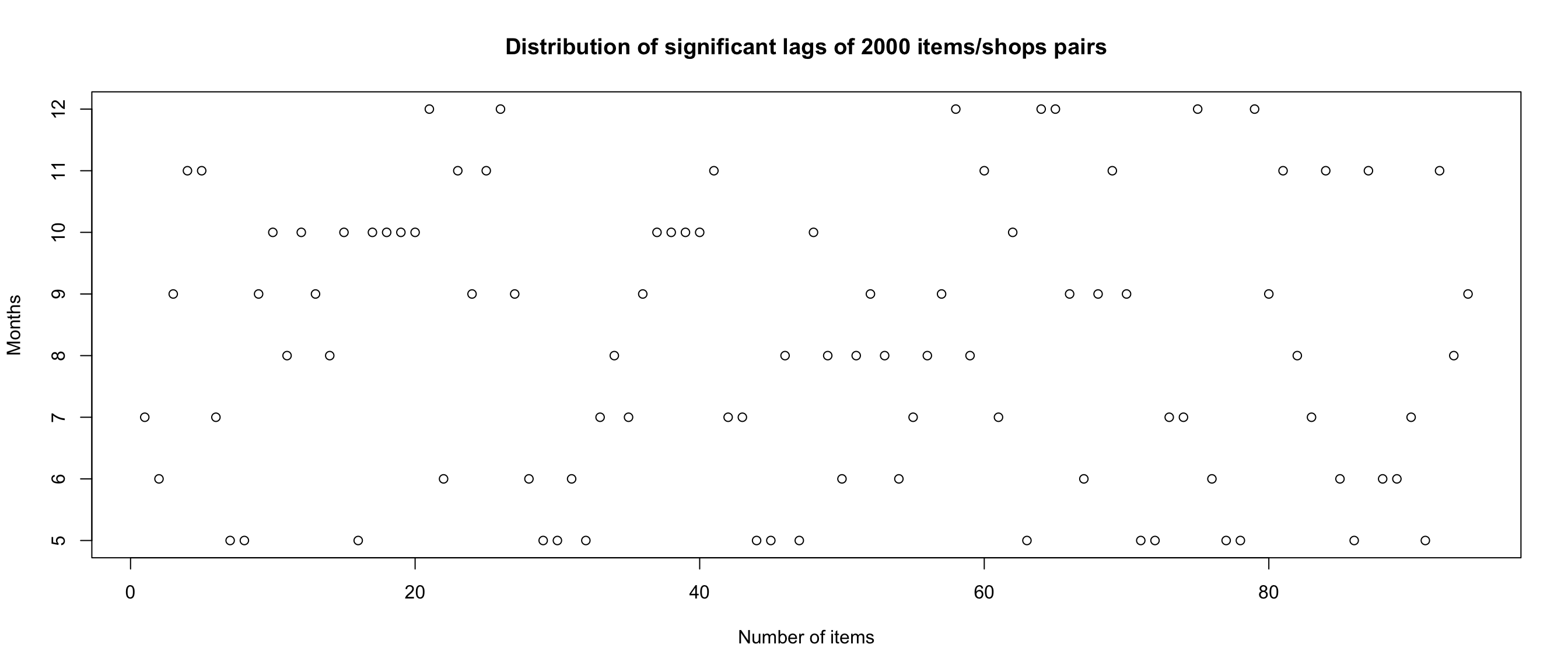
## [1] "Mean of significant lags is 8 Months"1 corresponds to 12 months. 0.67 ==> 12 * 0.67 = 8 Months
2.2 Visualize significant threshold (dashed blue line)
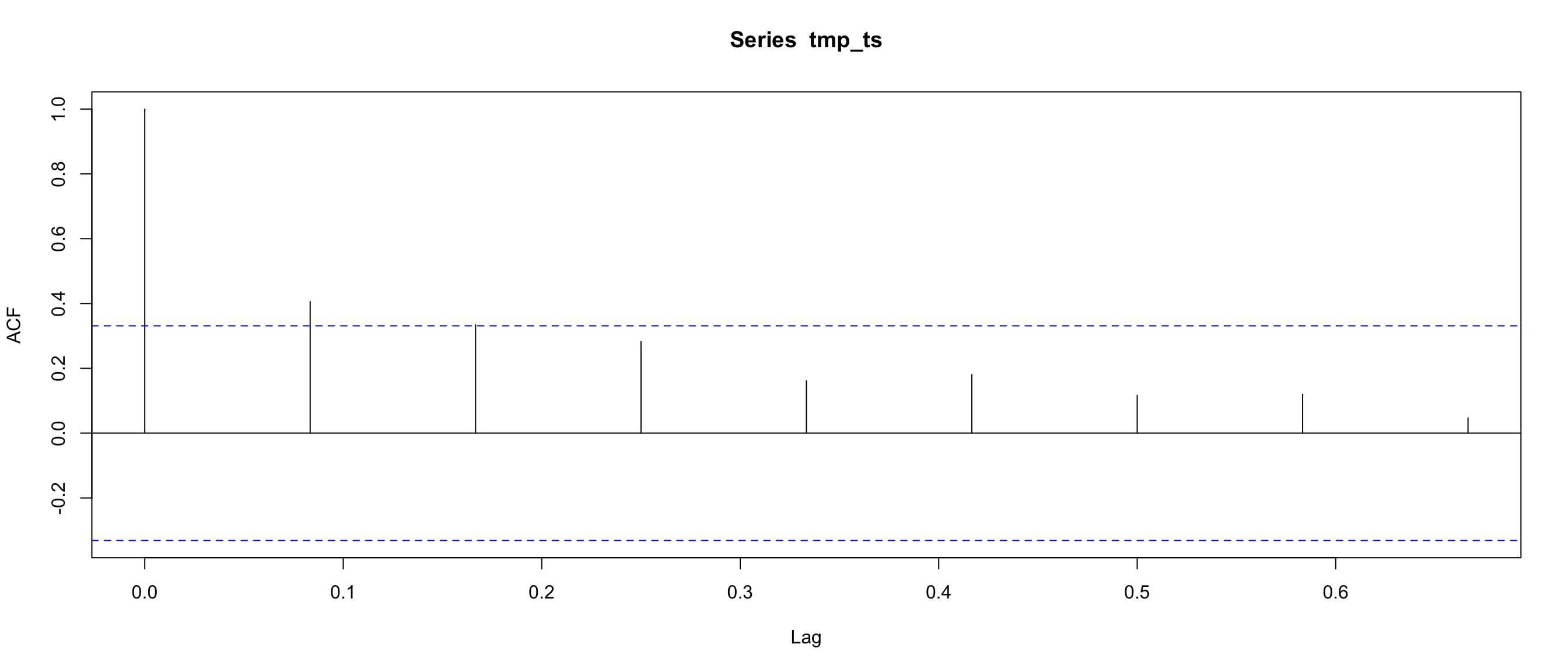
## [1] 0.083333332.3 add date and item_category_id columns to test dataset
test <- test %>% mutate(IDx = paste(shop_id, item_id, sep = "_"))
test["item_category_id"] <- NA
## add item_category_id from train
test <- train %>%
mutate(IDx = paste(shop_id, item_id, sep = "_")) %>%
full_join(test, by= c("shop_id","item_id" ,"IDx")) %>%
mutate(item_category_id = coalesce(as.integer(item_category_id.x), as.integer(item_category_id.y))) %>%
distinct(ID, .keep_all = TRUE) %>%
mutate(date_block_num = as.integer(34)) %>%
select(date_block_num, ID, IDx, item_id, shop_id, item_category_id) %>%
filter(!is.na(ID))
test %>% head## date_block_num ID IDx item_id shop_id item_category_id
## 1 34 150983 59_22154 22154 59 37
## 2 34 56520 25_2574 2574 25 55
## 3 34 56539 25_2607 2607 25 55
## 4 34 56666 25_2614 2614 25 55
## 5 34 57021 25_2808 2808 25 30
## 6 34 60179 25_2703 2703 25 302.4 Add ID to train dataset
train_only_ID <- train %>%
mutate(IDx = paste(shop_id, item_id, sep = "_")) %>%
full_join(test, by= c("shop_id","item_id" ,"IDx")) %>%
mutate(item_category_id = coalesce(as.integer(item_category_id.x), as.integer(item_category_id.y))) %>%
mutate(date_block_num = coalesce(as.integer(date_block_num.x), as.integer(date_block_num.y))) %>%
select(date_block_num, ID, IDx, shop_id, item_id, item_category_id, item_cnt_day, item_price) %>%
filter(!is.na(ID)) %>%
filter(date_block_num <34)
train_only_ID %>% summary## date_block_num ID IDx shop_id
## Min. : 0.00 Min. : 0 Length:1224439 Min. : 2.00
## 1st Qu.:12.00 1st Qu.: 47841 Class :character 1st Qu.:19.00
## Median :21.00 Median : 87160 Mode :character Median :31.00
## Mean :19.35 Mean : 95177 Mean :32.15
## 3rd Qu.:27.00 3rd Qu.:140099 3rd Qu.:46.00
## Max. :33.00 Max. :214199 Max. :59.00
## item_id item_category_id item_cnt_day item_price
## Min. : 30 Min. : 2.00 Min. : -16.000 Min. : 0.5
## 1st Qu.: 4181 1st Qu.:25.00 1st Qu.: 1.000 1st Qu.: 299.0
## Median : 7856 Median :38.00 Median : 1.000 Median : 549.0
## Mean : 9615 Mean :40.56 Mean : 1.321 Mean : 1030.7
## 3rd Qu.:15229 3rd Qu.:55.00 3rd Qu.: 1.000 3rd Qu.: 1199.0
## Max. :22167 Max. :83.00 Max. :2169.000 Max. :59200.03 Feature Engineering
3.1 Create lag and sliding window variables using the RcppRoll package
Before creating these new features, we must order the data set by date so the lag value is the previous date. There are a wide variety of statistical features we could create here. Here we will create three new features using the unit_sales column: lag_1 (1-day lag), 2 , 3, avg_1 (1-day rolling mean) and avg_2 (3-day rolling mean).
full <- train_only_ID %>%
full_join(test, by= c("ID","shop_id","item_id" ,"IDx", "item_category_id", "date_block_num")) %>%
select(date_block_num, ID, item_id, shop_id, item_cnt_day, item_price, item_category_id ) %>%
mutate(item_cnt_day = ifelse(item_cnt_day < 0, 0, item_cnt_day)) %>%
mutate(item_cnt_day = ifelse(item_cnt_day > 20, 20, item_cnt_day)) %>%
mutate(item_cnt_day = ifelse(is.na(item_cnt_day), 0, item_cnt_day)) %>%
mutate(item_price = ifelse(item_price < 0, 0, item_price)) %>%
mutate(item_price = ifelse(is.na(item_price), 0, item_price))
# Do scaling
#scale.cols <- c( "item_cnt_day", "item_price")
#full <- as.data.table(full)[, (scale.cols) := lapply(.SD, scale), .SDcols = scale.cols]
summary(full)## date_block_num ID item_id shop_id
## Min. : 0.00 Min. : 0 Min. : 30 Min. : 2.00
## 1st Qu.:14.00 1st Qu.: 48095 1st Qu.: 4240 1st Qu.:19.00
## Median :23.00 Median : 90620 Median : 8148 Median :31.00
## Mean :21.54 Mean : 96952 Mean : 9824 Mean :32.08
## 3rd Qu.:31.00 3rd Qu.:142857 3rd Qu.:15287 3rd Qu.:46.00
## Max. :34.00 Max. :214199 Max. :22167 Max. :59.00
##
## item_cnt_day item_price item_category_id
## Min. : 0.000 Min. : 0.0 Min. : 2.00
## 1st Qu.: 1.000 1st Qu.: 199.0 1st Qu.:28.00
## Median : 1.000 Median : 399.0 Median :40.00
## Mean : 1.096 Mean : 877.2 Mean :40.83
## 3rd Qu.: 1.000 3rd Qu.: 1000.0 3rd Qu.:55.00
## Max. :20.000 Max. :59200.0 Max. :83.00
## NA's :1027963.2 Data Cleansing
The evaluation metric of the competition is LRMSE (Log Root Mean Squared Error). The reason for using this metric is to scale the impact of inaccurate predictions. Using the log penalizes predicting 1 when the actual is 6 more than predicting 40 when the actual is 45. We convert unit_sales to log unit_sales here .
3.3 log1P transformation of train and merge with test
full_feature <- full %>%
dplyr::arrange(date_block_num) %>%
dplyr::group_by(shop_id, item_id, date_block_num, ID) %>% # , item_category_id)
dplyr::summarise(
target = log1p(sum(item_cnt_day, na.rm = TRUE)), # sclae with log1p
mean_price = log1p(mean(item_price, na.rm = TRUE)) # sclae with log1p
) %>%
dplyr::ungroup() %>%
dplyr::arrange(shop_id, item_id, date_block_num) %>% # , item_category_id)
dplyr::mutate(
last_sales1 = lag(target, 1),
last_sales2 = lag(target, 2),
last_sales3 = lag(target, 3),
#avg_1 = lag(RcppRoll::roll_meanr(target, 1), 1),
#last_sales4 = lag(target, 4),
last_price1 = lag(mean_price, 1),
#last_price2 = lag(mean_price, 2),
#last_price3 = lag(mean_price, 3),
last_sales1_3_mean = (last_sales1 + last_sales2 + last_sales3 )/3
) #%>%
#dplyr::filter(date_block_num == 34 - 1)
summary(full_feature)## shop_id item_id date_block_num ID
## Min. : 2.00 Min. : 30 Min. : 0.0 Min. : 0
## 1st Qu.:18.00 1st Qu.: 4628 1st Qu.:17.0 1st Qu.: 49837
## Median :31.00 Median : 9974 Median :26.0 Median : 97989
## Mean :31.95 Mean :10279 Mean :23.8 Mean :100797
## 3rd Qu.:47.00 3rd Qu.:15512 3rd Qu.:34.0 3rd Qu.:147626
## Max. :59.00 Max. :22167 Max. :34.0 Max. :214199
##
## target mean_price last_sales1 last_sales2
## Min. :0.0000 Min. : 0.000 Min. :0.0000 Min. :0.0000
## 1st Qu.:0.0000 1st Qu.: 0.000 1st Qu.:0.0000 1st Qu.:0.0000
## Median :0.6931 Median : 5.704 Median :0.6931 Median :0.6931
## Mean :0.7500 Mean : 4.633 Mean :0.7500 Mean :0.7500
## 3rd Qu.:1.0986 3rd Qu.: 6.685 3rd Qu.:1.0986 3rd Qu.:1.0986
## Max. :6.4281 Max. :10.669 Max. :6.4281 Max. :6.4281
## NA's :1 NA's :2
## last_sales3 last_price1 last_sales1_3_mean
## Min. :0.0000 Min. : 0.000 Min. :0.0000
## 1st Qu.:0.0000 1st Qu.: 0.000 1st Qu.:0.4621
## Median :0.6931 Median : 5.704 Median :0.6931
## Mean :0.7500 Mean : 4.633 Mean :0.7500
## 3rd Qu.:1.0986 3rd Qu.: 6.685 3rd Qu.:0.9635
## Max. :6.4281 Max. :10.669 Max. :6.4067
## NA's :3 NA's :1 NA's :33.4 Split train and test
test_feature <- full_feature %>% #
select(date_block_num, shop_id, item_id, target, everything()) %>% # last_sales1_4_mean item_category_id ,
dplyr::arrange(date_block_num) %>%
filter(date_block_num == c(34))
train_feature <- full_feature %>%
select(date_block_num, shop_id, item_id, target, everything()) %>% #last_sales1_4_mean, item_category_id ,
dplyr::arrange(date_block_num) %>%
filter(date_block_num < 34) # ytrain <- train_feature$target
# ytest <- test_feature$target
#
# xtrain <- train_feature %>% select(-target) %>% as.matrix()
#
# xtest <- test_feature %>% select(-target) %>% as.matrix()
#
# #preparing matrix
# dtrain <- xgb.DMatrix(data = new_tr,label = labels)
# dtest <- xgb.DMatrix(data = new_ts,label=ts_label)
#
# # calculate modeling
# xgb <- xgboost(data = xtrain,
# label = ytrain,
# booster = "gbtree",
# objective = "reg:linear",
# eval_metric = "rmse",
# eta = 0.1,
# max_depth = 6,
# nround=10,
# nthread = 3)3.5 Xgboost Modeling
target <- train_feature$target
ID <- test$ID
#Returns object unchanged if there are NA values
previous_na_action<- options('na.action')
options(na.action='na.pass')
trainMatrix <- sparse.model.matrix(target ~ last_sales1 + item_id + last_price1 + last_sales1_3_mean , # + item_category_id + avg_1 last_sales2
data = train_feature,
contrasts.arg = c( 'ID', 'item_id', 'shop_id'),
sparse = TRUE, sci = FALSE) #, 'item_category_id'
#contrasts.arg = lapply(train_feature[,c('ID','shop_id', 'item_id')], contrasts,
# contrasts=FALSE),sparse = FALSE, sci = FALSE)
#Create input for xgboost
trainDMatrix <- xgb.DMatrix(data = trainMatrix, label = train_feature$target)
testMatrix <- sparse.model.matrix(target ~ last_sales1 + item_id + last_price1 + last_sales1_3_mean, # item_category_id + avg_1 last_sales2
data = test_feature,
contrasts.arg = c('ID' ,'shop_id', 'item_id'), #, 'item_category_id'
sparse = TRUE, sci = FALSE)
#Create input for xgboost
testDMatrix <- xgb.DMatrix(data = testMatrix, label = test_feature$target)
params <- list(booster = "gbtree",
objective = "reg:linear",
eval_metric = "rmse",
eta=0.5, # 58 round train-rmse:0.347514+0.000495 test-rmse:0.372750+0.001166
# gamma=1, # [79] train-rmse:0.322082+0.000747 test-rmse:0.354592+0.000740 (Best score)
max_depth = 10,
subsample = 0.5,
min_child_weight = 5
)
library(parallel)
# parallel calculation
N_cpu = parallel::detectCores()
#Cross-validation
xgb.tab <- xgb.cv(data = trainDMatrix,
param = params,
maximize = FALSE, nrounds = 1000,
nthreads = N_cpu, nfold = 5, early_stopping_round = 10)## [1] train-rmse:0.516012+0.000891 test-rmse:0.517630+0.003108
## Multiple eval metrics are present. Will use test_rmse for early stopping.
## Will train until test_rmse hasn't improved in 10 rounds.
##
## [2] train-rmse:0.435514+0.000774 test-rmse:0.438714+0.002929
## [3] train-rmse:0.409573+0.001347 test-rmse:0.414219+0.002265
## [4] train-rmse:0.399635+0.000927 test-rmse:0.405059+0.002169
## [5] train-rmse:0.394350+0.001757 test-rmse:0.400662+0.002541
## [6] train-rmse:0.391375+0.001480 test-rmse:0.398490+0.002178
## [7] train-rmse:0.388660+0.001083 test-rmse:0.396448+0.001947
## [8] train-rmse:0.385769+0.001225 test-rmse:0.394178+0.002705
## [9] train-rmse:0.383128+0.001945 test-rmse:0.392261+0.003139
## [10] train-rmse:0.381510+0.001755 test-rmse:0.391279+0.003550
## [11] train-rmse:0.379617+0.002212 test-rmse:0.389929+0.003702
## [12] train-rmse:0.378540+0.002196 test-rmse:0.389280+0.003375
## [13] train-rmse:0.377392+0.002258 test-rmse:0.388628+0.003234
## [14] train-rmse:0.376188+0.001665 test-rmse:0.387894+0.002929
## [15] train-rmse:0.375180+0.002018 test-rmse:0.387240+0.003285
## [16] train-rmse:0.374306+0.001974 test-rmse:0.386788+0.003534
## [17] train-rmse:0.371896+0.001347 test-rmse:0.384948+0.003200
## [18] train-rmse:0.370831+0.001660 test-rmse:0.384265+0.002930
## [19] train-rmse:0.370087+0.001519 test-rmse:0.383978+0.003026
## [20] train-rmse:0.368921+0.001118 test-rmse:0.383225+0.002837
## [21] train-rmse:0.368233+0.001162 test-rmse:0.382855+0.002751
## [22] train-rmse:0.367214+0.001219 test-rmse:0.382291+0.002451
## [23] train-rmse:0.366442+0.001234 test-rmse:0.381852+0.002342
## [24] train-rmse:0.365832+0.001193 test-rmse:0.381622+0.002585
## [25] train-rmse:0.365389+0.001068 test-rmse:0.381609+0.002448
## [26] train-rmse:0.364561+0.001242 test-rmse:0.381202+0.001958
## [27] train-rmse:0.364155+0.001273 test-rmse:0.381115+0.001918
## [28] train-rmse:0.363786+0.001375 test-rmse:0.381156+0.001928
## [29] train-rmse:0.363276+0.001340 test-rmse:0.381089+0.001981
## [30] train-rmse:0.362941+0.001348 test-rmse:0.381087+0.001977
## [31] train-rmse:0.362629+0.001337 test-rmse:0.381018+0.001932
## [32] train-rmse:0.362214+0.001450 test-rmse:0.380847+0.002026
## [33] train-rmse:0.361702+0.001646 test-rmse:0.380710+0.001915
## [34] train-rmse:0.361171+0.001803 test-rmse:0.380554+0.001862
## [35] train-rmse:0.360655+0.001591 test-rmse:0.380316+0.001846
## [36] train-rmse:0.359948+0.001462 test-rmse:0.380020+0.001732
## [37] train-rmse:0.359449+0.001511 test-rmse:0.379818+0.001643
## [38] train-rmse:0.359057+0.001639 test-rmse:0.379810+0.001632
## [39] train-rmse:0.358649+0.001550 test-rmse:0.379803+0.001640
## [40] train-rmse:0.358428+0.001600 test-rmse:0.379852+0.001614
## [41] train-rmse:0.358094+0.001651 test-rmse:0.379832+0.001501
## [42] train-rmse:0.357515+0.001441 test-rmse:0.379596+0.001489
## [43] train-rmse:0.356958+0.001471 test-rmse:0.379332+0.001652
## [44] train-rmse:0.356677+0.001542 test-rmse:0.379276+0.001547
## [45] train-rmse:0.356331+0.001462 test-rmse:0.379243+0.001536
## [46] train-rmse:0.355979+0.001494 test-rmse:0.379124+0.001683
## [47] train-rmse:0.355555+0.001543 test-rmse:0.379093+0.001635
## [48] train-rmse:0.355043+0.001500 test-rmse:0.378898+0.001587
## [49] train-rmse:0.354500+0.001602 test-rmse:0.378684+0.001490
## [50] train-rmse:0.354010+0.001458 test-rmse:0.378441+0.001646
## [51] train-rmse:0.353584+0.001382 test-rmse:0.378390+0.001601
## [52] train-rmse:0.353185+0.001478 test-rmse:0.378325+0.001363
## [53] train-rmse:0.352879+0.001483 test-rmse:0.378236+0.001295
## [54] train-rmse:0.352544+0.001491 test-rmse:0.378255+0.001324
## [55] train-rmse:0.352156+0.001495 test-rmse:0.378213+0.001443
## [56] train-rmse:0.351797+0.001470 test-rmse:0.378273+0.001457
## [57] train-rmse:0.351435+0.001467 test-rmse:0.378287+0.001468
## [58] train-rmse:0.350944+0.001563 test-rmse:0.378095+0.001399
## [59] train-rmse:0.350676+0.001562 test-rmse:0.378125+0.001360
## [60] train-rmse:0.350280+0.001457 test-rmse:0.378014+0.001434
## [61] train-rmse:0.350041+0.001542 test-rmse:0.378065+0.001440
## [62] train-rmse:0.349771+0.001485 test-rmse:0.378130+0.001473
## [63] train-rmse:0.349459+0.001445 test-rmse:0.378099+0.001540
## [64] train-rmse:0.349247+0.001426 test-rmse:0.378102+0.001496
## [65] train-rmse:0.349019+0.001457 test-rmse:0.378179+0.001529
## [66] train-rmse:0.348682+0.001426 test-rmse:0.378198+0.001443
## [67] train-rmse:0.348483+0.001435 test-rmse:0.378241+0.001406
## [68] train-rmse:0.348162+0.001424 test-rmse:0.378256+0.001324
## [69] train-rmse:0.347805+0.001358 test-rmse:0.378256+0.001317
## [70] train-rmse:0.347543+0.001337 test-rmse:0.378333+0.001308
## Stopping. Best iteration:
## [60] train-rmse:0.350280+0.001457 test-rmse:0.378014+0.001434#Number of rounds
num_iterations = xgb.tab$best_iteration
xgboost_tree <- xgb.train(data = trainDMatrix
, param = params
, maximize = FALSE, evaluation = 'rmse', nrounds = num_iterations)
## xgb.train is an advanced interface for training an xgboost model.
## The xgboost function is a simpler wrapper for xgb.train.
# # modling
# set.seed(17)
#model_xgb <- xgboost(param = params, data = as.matrix(select(train_feature, -target )), label = train_feature$target ,
# nrounds = which.min(xgb.tab$evaluation_log$test_rmse_mean),
# nthread = N_cpu, importance = TRUE)
#xgb.importance(model = xgboost_tree)
importance <- xgb.importance(feature_names = colnames(trainMatrix), model = xgboost_tree)
ggplotly(xgb.ggplot.importance(importance_matrix = importance))3.6 Prediction
## Min. 1st Qu. Median Mean 3rd Qu. Max.
## 0.2124 0.7792 0.8270 0.8896 0.9048 6.1109## Min. 1st Qu. Median Mean 3rd Qu. Max.
## 1.237 2.180 2.286 2.550 2.471 450.740submission1 <- data.frame(
ID = ID,
item_cnt_month = pred_tree
)
submission_scale %>% arrange(ID) %>% summary## Error in eval(lhs, parent, parent): object 'submission_scale' not found3.7 Setting params with mlr package 
# library(mlr)
# Train_mlr <- as.data.frame(train_with_features)
# Test_mlr <- as.data.frame(Test)
#
# ## store Id column and remove it from the train and test data
# Test_mlr['item_cnt_month'] <- 0
#
# testId = Test_mlr$ID
# Train_mlr$ID = Test_mlr$ID = NULL
#
# Train_mlr$IDx <- as.factor(Train_mlr$IDx)
# Test_mlr$IDx <- as.factor(Test_mlr$IDx)
# ## create mlr task and convert factors to dummy features
# trainTask = makeRegrTask(data = Train_mlr, target = "item_cnt_month")
# trainTask = createDummyFeatures(trainTask)
# testTask = makeRegrTask(data = Test_mlr, target = "item_cnt_month")
# testTask = createDummyFeatures(testTask)
#
#
# ## Error: vector memory exhausted (limit reached?)4 Notes: Parameters versus Features importance plots
I tried to understand how can tune xgboost parameters to get best rmse score.
4.1 How to plot feature importance with ggplot
## Warning in cluster.1d.dp(x, k, y, method, estimate.k, "L2", deparse(substitute(x)), : Max number of clusters is greater than the unique number of
## elements in the input vector, and k.max is set to the number of
## unique number of input values.Clusters <- clusters$cluster %>% as.character() %>% as.factor()
tex <- paste0("eta = 0.5,\nmax_depth = 11,\nsubsample = 1,\nmin_child_weight = 5" )
importance %>%
ggplot() +
aes(x = reorder(Feature, Importance), y = Importance , fill =Clusters ) +
geom_col() +
coord_flip() +
geom_text(x=6, y=0.2, label=tex, hjust = 'left') +
labs(title = "score = 1.29")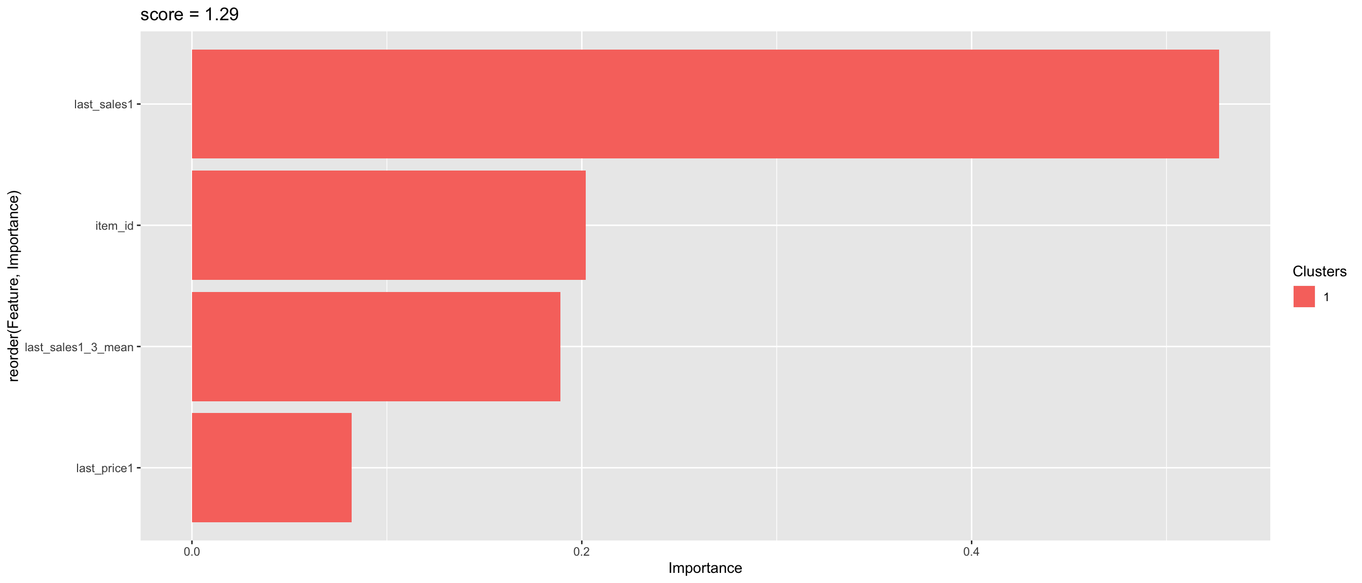
5 Naive forecasting from this kernel
train %>%
mutate(IDx = paste(shop_id, item_id, sep = "_")) %>%
left_join(test, by= c("shop_id","item_id" )) %>%
select(date, date_block_num ,shop_id, item_id, ID, item_cnt_day) %>%
na.omit(ID) %>%
dplyr::group_by(shop_id, item_id, date_block_num) %>%
dplyr::summarise(total_num_sales = sum(item_cnt_day, na.rm = TRUE)) %>%
dplyr::ungroup() %>%
dplyr::filter((date_block_num == 33)) %>%
dplyr::mutate(item_cnt_month = ifelse((total_num_sales < 0), 0,
ifelse(total_num_sales > 20, 20, total_num_sales))) %>%
dplyr::left_join(test, by = c("shop_id", "item_id")) %>%
dplyr::select(ID, item_cnt_month) %>% head## Error in .f(.x[[i]], ...): object 'date_block_num' not found